

The minimal coupled field system defining the dynamical backbone of HGUT.
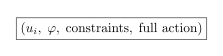
The HGUT Master Lagrangian
I. Ontological Basis
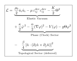
HGUT models the vacuum as a continuous, non-dissipative medium with two fundamental degrees of freedom: a displacement field and an internal scalar field.


The displacement field describes the mechanical configuration of the medium and obeys linear elasticity at lowest order. The scalar field is Klein–Gordon-like. Its local oscillation rate supplies an emergent clock variable, but the scalar itself is a dynamical field rather than a phase angle.
Field-content status
This chapter uses a strictly real scalar field to establish the classical dynamical baseline. The complex extension is introduced separately when constructing a conserved phase-sector density.
II. Kinematic Definitions
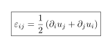
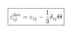
The elastic sector is described by the linear strain tensor, volumetric strain, and deviatoric strain.


III. Action Principle
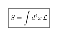
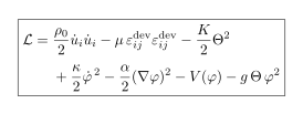
The dynamics are defined by an action built from the smooth-sector Lagrangian.
Assumptions and constraints
- The coefficients ρ₀, μ, K, κ, and α are strictly positive.
- No dissipative terms are present.
- The coupling constant has dimensions set by the bulk modulus and the scalar-field normalization.
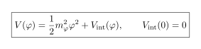
- The scalar potential is bounded below and at least quadratic near the origin.
Sign audit
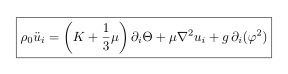
For the interaction term −gΘφ², variation with respect to the displacement field produces the mechanical source +g∂ᵢ(φ²). A minus sign in the displacement equation would be inconsistent with the action.
Stability of the static energy
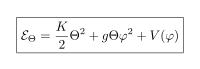
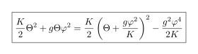
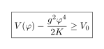
A sufficient condition is that the quartic contribution in the scalar potential dominate the induced negative quartic term.
Symmetries of the action
- Spatial translations and rotations.
- Time translation.
- Internal ℤ₂ symmetry under φ → −φ, provided the potential is even.
- Galilean boost structure at the elastic level. Bare Lorentz invariance is not assumed.
IV. Topological Sector — Deferred
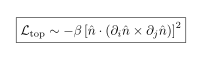
The smooth action supports wave-like excitations but does not by itself guarantee stable, finite-energy, topologically protected particle-like solutions. A genuine topological sector requires a director or normalized configuration field and a term of Faddeev–Skyrme type, or an equivalent construction admitting a Hopf invariant.
Status
The explicit topological sector is deferred. The remainder of this chapter treats only the smooth elastic and scalar sectors.
V. Field Equations
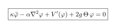
Variation of the smooth-sector action with respect to the displacement and scalar fields yields the coupled system below.
Displacement equation
Phase equation
Interpretation
- Volumetric strain acts as an effective mass-squared correction for the scalar field and changes its local oscillation rate.
- Spatial gradients of φ² source the displacement field through the corrected term +g∂ᵢ(φ²).
- Both effects arise from the single scalar interaction −gΘφ².
VI. Propagation Speeds and the Lorentz Question
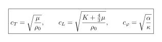
In the uncoupled linearized limit, the elastic and scalar sectors possess three distinct characteristic speeds.
Open requirement
A physically complete theory must explain how observable excitations share a single effective limiting speed. The bare smooth-sector action does not establish this.
Candidate mechanisms include suppression or gapping of the longitudinal sector, deeper parameter relations, or a restriction of observable matter to a selected propagation sector.
VII. Local Clock from the Phase Sector
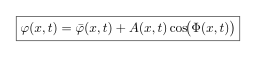
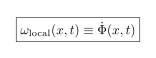
In a region where the scalar oscillates approximately harmonically about a slowly varying background, write:
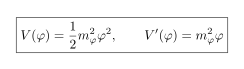
Near a strictly quadratic vacuum potential:
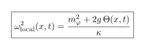
The linearized phase equation gives the strain-shifted local oscillation frequency:
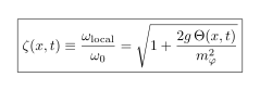
Relative to the unperturbed frequency, define the Harrison clock factor:
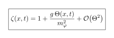
In the weak-strain regime:
The operational accumulated phase along a trajectory is:
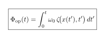
With the convention Θ > 0 for dilation and Θ < 0 for compression, the sign of the coupling determines whether dilation raises or lowers the local oscillation rate. The physical sign of the coupling and the gravitational strain profile remain separate dynamical questions.
VIII. Initial-Value Formulation
The coupled system is second order in time. A well-posed initial-value problem requires the displacement, displacement velocity, scalar field, and scalar velocity on a Cauchy surface.

No further constraints are present in the unconstrained smooth formulation. An incompressibility condition would require a Lagrange multiplier and would alter the displacement equation.
IX. Structural Summary
- Navier–Cauchy-type elastic dynamics for the displacement field.
- Klein–Gordon-type dynamics for the real scalar field.
- Bidirectional coupling through −gΘφ².
- A derived local clock variable from the scalar oscillation rate.
- A deferred topological sector required for stable knot excitations.
X. Structural Status and Program Forward
Established here
- A non-dissipative action principle.
- A coupled displacement and scalar field system derived from that action.
- A mechanically interpretable scalar coupling.
- A well-defined initial-value formulation.
- A local clock factor derived from phase-sector dynamics.
Deferred structures
- The complex phase extension and U(1) current.
- The Born density and Schrödinger envelope limit.
- The topological Harrison-knot sector.
- The Bell-sector corridor and holonomy structure.
Nothing new is postulated beyond this point. The later structure is extracted through controlled extensions and reductions of this dynamical backbone.
Derivation from the Action
The coupled equations follow from the Euler–Lagrange equations applied separately to the displacement and scalar fields.
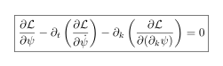
Variation with respect to the displacement field
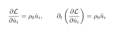
Kinetic term
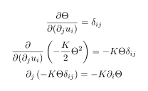
Bulk volumetric-strain term
Deviatoric elastic term
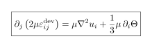
Coupling term
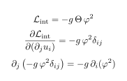
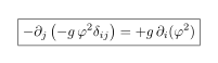
The Euler–Lagrange equation contains the negative divergence of the spatial derivative term. That collection step changes the displayed sign of the mechanical source:
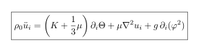
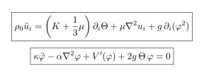
Collecting the inertial, elastic, volumetric, and coupling terms gives:
Variation with respect to the scalar field
Kinetic term
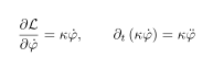
Gradient term
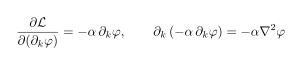
Potential and coupling terms
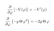
Collecting all scalar terms gives:
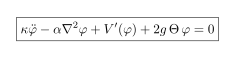
Coupling consistency
The scalar sources the mechanical field through +g∂ᵢ(φ²), while volumetric strain enters the scalar equation through +2gΘφ on the left-hand side. Both arise from one interaction term.

Minimal smooth-sector equations
Consistency Checks
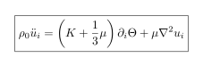
Elastic limit
Setting the scalar field and coupling to zero recovers the isotropic Navier–Cauchy equation.
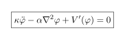
Scalar-field limit
Setting the displacement field and volumetric strain to zero gives the decoupled scalar equation.
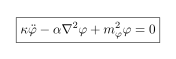
For a quadratic potential, this becomes a Klein–Gordon-type wave equation.
Coupled-medium limit
For nonzero coupling, volumetric strain shifts the local scalar oscillation rate while gradients of scalar intensity source mechanical stress.
Status and Role in the Volume
This chapter establishes the classical real-scalar baseline of HGUT. It defines the smooth coupled medium dynamics from which the complex phase extension, quantum envelope limit, measurement dynamics, and topological sector are subsequently constructed.